
How do drone photos become decisions on your network? Fly to a plan, send us the photos, we process them on our own servers, and the result comes back as a map, tables and marked photos. LiDAR point clouds run in the same chain.
Upload with your upload code, we run the analysis on our side, and the processed result comes back to your browser. No installation, no fee.
Photo passport, detection, poles, network and report.
Start the photo test →10 daysLiDAR · LAS / LAZUpload your point cloudCorridor cut, classification, clearance and fall-in risk, map and 3D.
Start the LiDAR test →The photos decide what the AI can see. The guide shows the automated flight plan in 3D, step by step: three orbits and the detail shots, per drone camera, for medium and high voltage, with the flight time and every photo the drone takes.
This is our recommendation. Every network and every drone fleet is different: contact us, and we tailor the flight plan to your lines, poles and cameras.
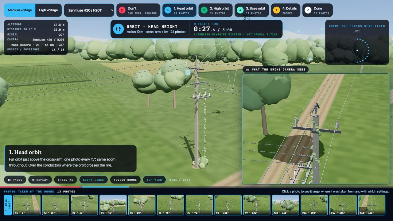 ▶ 3D flight plan
Bring the drone you already fly. The flight plan and the camera settings adapt to it.
Hovering in one spot and zooming is not enough: machine vision needs every part from many sides, at the same scale. So the drone flies three orbits at a fixed zoom, then the details.
Pick your camera; the flight and the settings follow it.
▶ Start the 3D flight planCamera settings per drone, the flight table, delivery and the on-site checklist.
Open the capture guidePhotos and point clouds go in through the same kind of secure upload, with one upload code. Your photos are processed on our own servers.
Watch one real photo package go through: real drone photos, the real grouping into poles, the real detections.
You get a personal code. With it, upload JPEG photos or a whole folder; they are packed in your browser.
Sent in parts over an encrypted relay. An interrupted upload resumes where it stopped.
Only real JPEGs pass. Duplicates are dropped; a photo set already processed is not processed again.
An operator approves every job before processing starts.
On our servers. Progress shows live in your browser.
Opens with your job number. AI results are marked as AI.
Where it was taken, with what, how sharp it is, and which inspection points it shows.
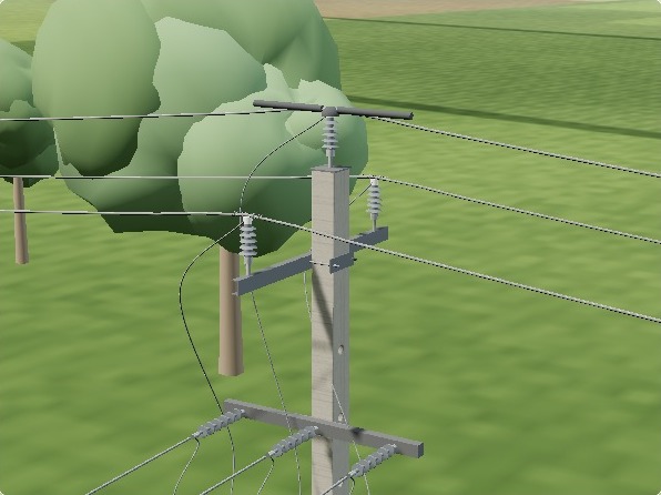
Send the network of the area with the photos. The principle: each photographed pole is matched to its line and its asset ID.
Public mapNo file? We use OpenStreetMap: line km by voltage, poles and branch points along your route.
No mapNo network here at all? The photographed poles are connected as an inferred route, marked as such.
Lines and poles with their IDs. Coordinates in WGS84 or your national grid; a file without a coordinate system is placed from the photo positions.
Self-service, from the first free test to the production system: you upload, the analysis runs, the result is in your browser.
The base price is in euro. US dollar amounts are approximate, converted at about $1.13 per €1.
You pay per pole, not per photo. Upload as many photo packages per pole as you need: repeat flights, new seasons, detail shots. Only the number of poles in your network counts.
A box on a photo is only the visible end. The principle: every point on the structure has its parts, what they are made of, the defects that can occur there, how each defect is seen and what it is confused with. This is what is taught, checked and reported, for distribution and transmission alike. Click a point.
From pixels to assets, in principle: detection on the photos, LiDAR for the corridor, a 3D model of the structure, matching to poles and the network, and a defect dictionary behind the findings.
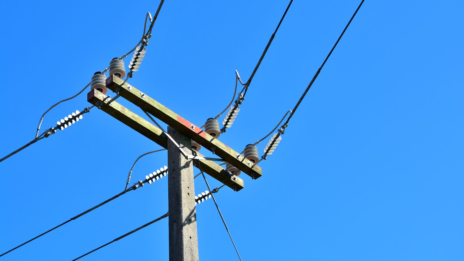
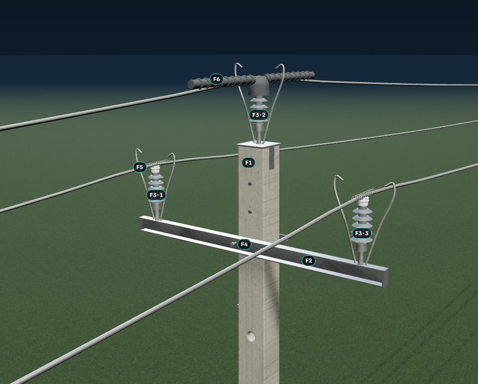
The principle: detection runs on the photos and marks components such as insulators, cross-arms, switches and the pole itself. Drag the line.
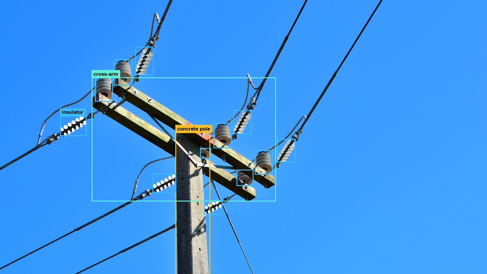 PhotoDetected
This picture shows the idea. In a project, what is detected and how it is evaluated is agreed with you: components matched across photos and poles, and defects described by the dictionary.
The idea: an inventory built from the photos, at component level: what is on each pole, and where.
Where real cases are rare, defects can be reproduced with today's technology, so a handful of examples is enough to train on.
A defect is a difference from what should be there. The asset database is what the difference is measured against.
Seen on the photos · three basic typesMeasured
A warning sign, the pole number. One or two sharp photos settle it.
A structure or any foreign object that can disturb the network: a nest, debris caught on the line, an attachment that does not belong.
The part is in place but looks different from the reference: broken, hanging, cracked, burnt.
Vegetation against the position of the network, conductor sag, a leaning pole. Not recognised from looks, measured.
An airborne LiDAR scan goes through the same steps: upload with a code, checks, approval, processing. Only the line corridor is processed.
In a projected coordinate system; read from the file, nothing to enter.
Only the points near the line are kept, before anything else runs.
Ground, vegetation, buildings, conductors and poles.
Trees with heights, clearance zones and fall-in risk, measured against the line.
Risk per span along the line, the point cloud in 3D and a decision report.
The two do different jobs, and meet on the same network: the line, the span, the pole.
Every structure type has its inspection points. Each point has its own list of possible defects. Every finding lands on a point of a pole, so it can be compared across photos, poles and years.
The photos are grouped into poles, the components into an object list, and the poles into your network.
Grouped by position: one pole per 30 m.
Material and function suggested from the components.
Counted on the photos, per class.
Network pole 6.1 m away, line and branch points checked.
Asset ID, components, grade.
Every finding comes from a dictionary: object → what decides it → defect → severity. Each defect says how it is seen and whether the AI can find it today.
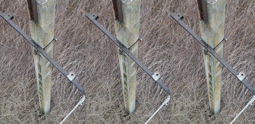
A crack across a concrete pole is rare in the photos, so we generate it: on real photos, with the width and direction set from the dictionary, and labelled automatically. The models learn it before the first one is reported.
The AI pre-labels everything. People accept or correct it, split by class. Until then, every result is marked as an AI result.
Full 3D capture — the most accurate 3D model from images. Full defect detection needs 16 photos per pole: 8 around the top, 8 around the base.
The result opens in your browser: a grade, a map with layers, the network, pole cards, tables and the marked photos.


An honest grade: these test photos were taken by hovering and zooming, so the report says they are not fit for defect assessment yet, and why.
You hand over photos. The aim is not a pile of photos to look through, but poles assessed, the finding behind each, the action it needs, and a work list in priority order.
| # | Pole | Component | Finding | Severity | Action |
|---|
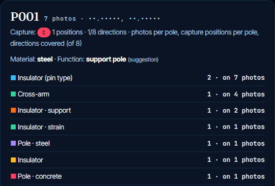
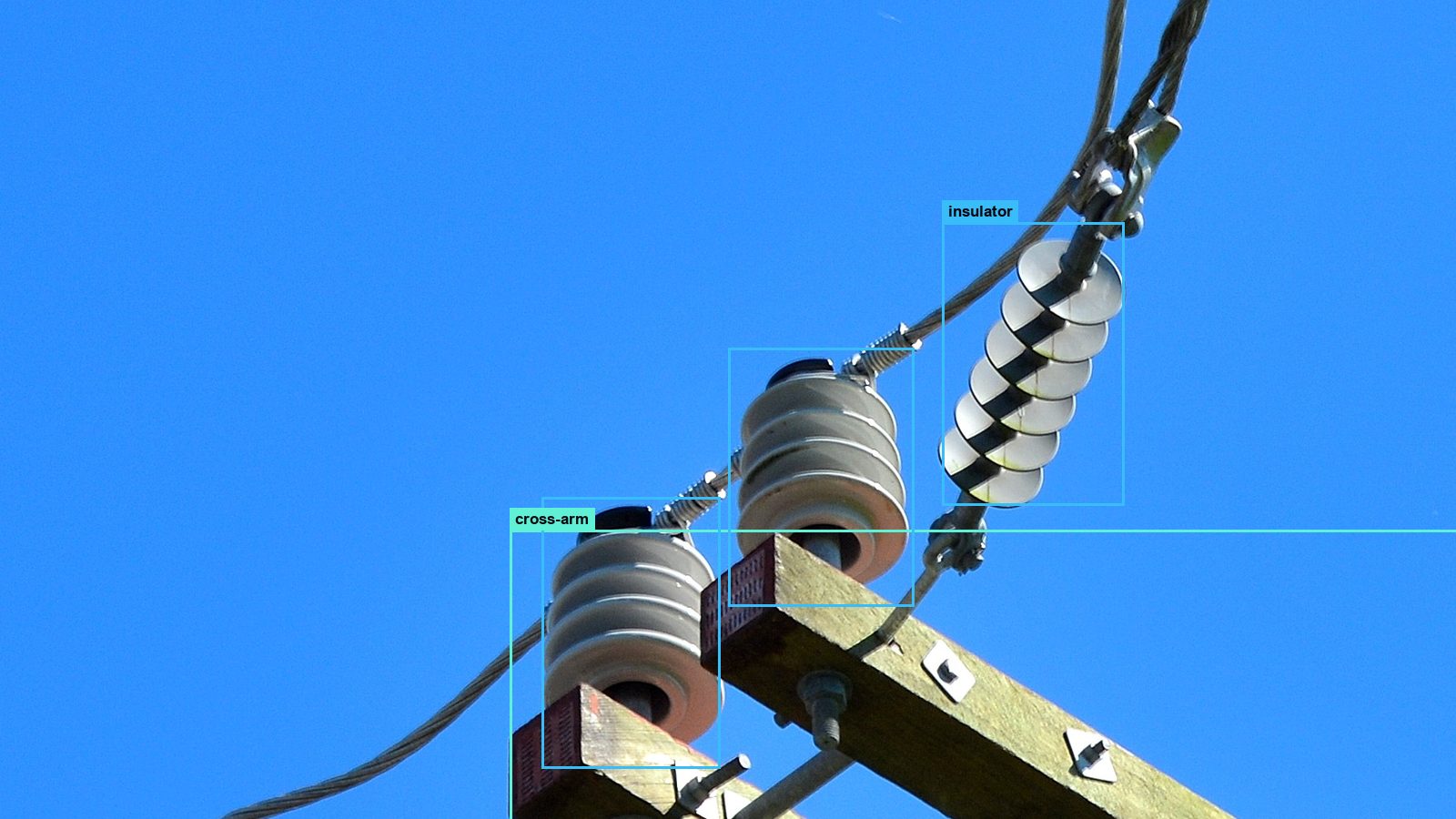
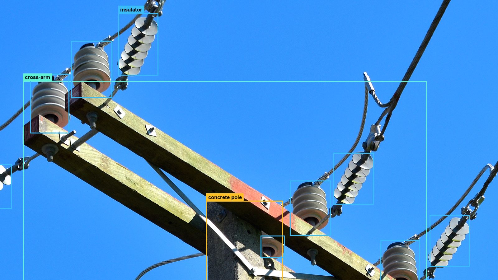
Each pole: grade, suggested material and function, the components with the number of photos they are on, and the photos themselves, marked.
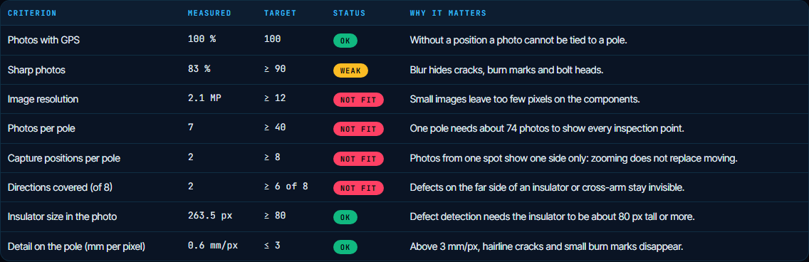
Fully free · upload your own drone photos or LiDAR point cloud.